
Crude oil production model
Model description
The Energy Futures Modeling System uses three distinct approaches to model crude oil production, designed to capture the characteristics of the different ways crude oil is produced in Canada. These are:
- Oil sands production
- Western Canada conventional, tight, and shale oil production
- Newfoundland and Labrador offshore oil production
Oil sands production
Figure OS.1: Oil sands model overview

Source and Description
Source: CER
Description: The infographic provides a simplified overview of the Oil Sands Model. The goal of the model is to project total oil sands production in a given year. Oil sands production is estimated on a project-by-project basis to determine future bitumen production, including future synthetic crude oil production and future diluted bitumen production. The model breaks these down into cost of production and status (producing or shut in).
Oil sands production categories
The oil sands model compiles historical oil sands production and projects future oil sands production on a project-by-project basis. Production is grouped by the categories each project belongs to (in situ, mined, or primary) and by end products (diluted bitumen or synthetic crude oil). Currently, most raw bitumen produced from mines is upgraded within Alberta to synthetic crude oil along with about 10% of in-situ production. Most of the in-situ production, as well as production from Imperial’s Kearl Mine and Suncor’s Fort Hills Mine, are marketed as diluted bitumen.
Figure OS.2: Oil sands production categories
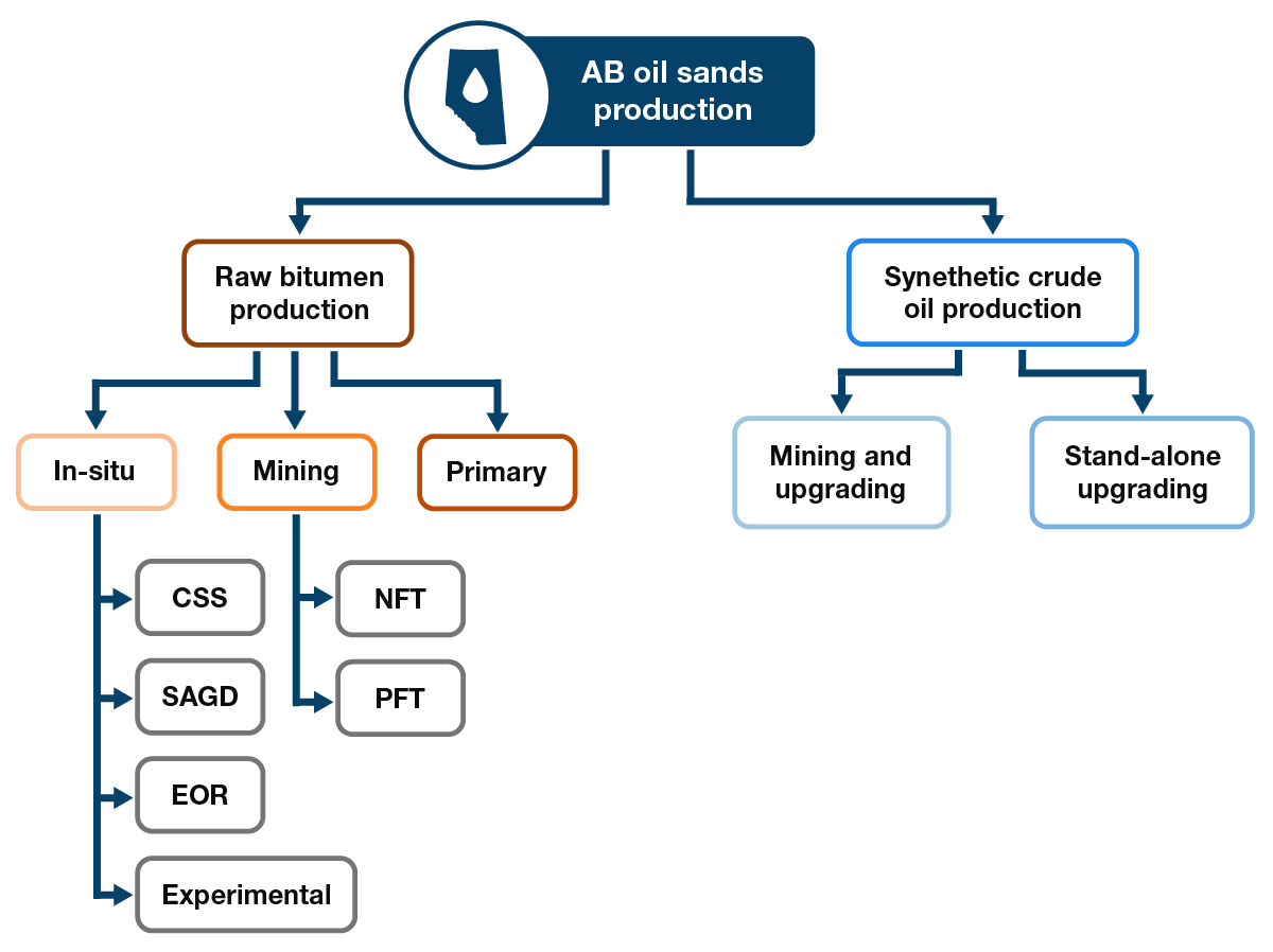
Source and Description
Source: Government of Alberta
Description: This flow chart shows the main products of oil sands production. Raw bitumen is produced through in-situ, mining, or primary production. In-situ production includes CSS, SAGD, EOR, and certain experimental schemes. Mining includes naphthenic froth treatment and paraffinic froth treatment production. Raw bitumen may then be upgraded into synthetic crude oil at either integrated mining and upgrading facilities or at stand-alone upgraders.
Figure OS.3: Oil sands areas map
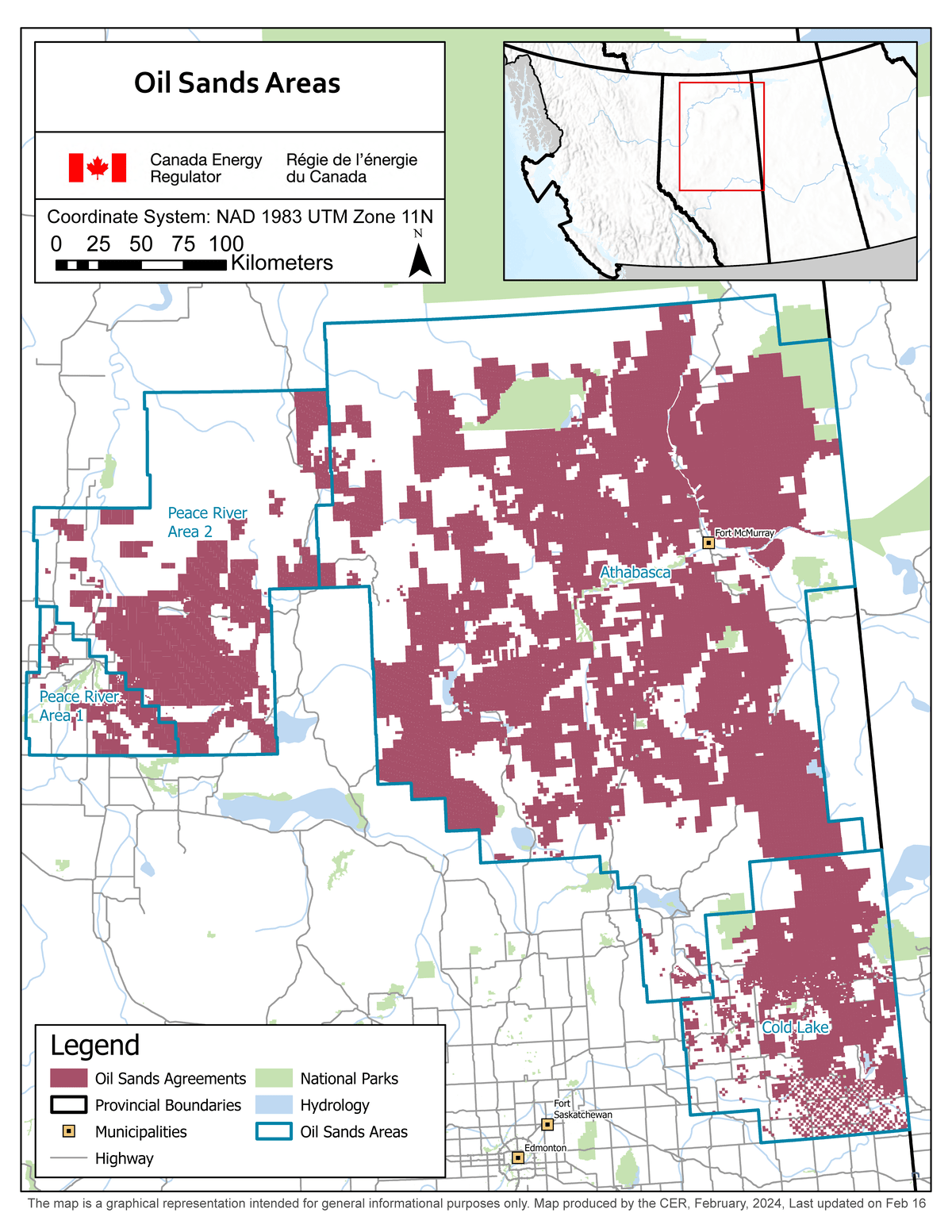
Source and Description
Source: Government of AlbertaFootnote 1
Description: This is a map that shows the amount of land leased in the three major oil sands areas; Athabasca, Peace River, and Cold Lake. Athabasca is the largest oil sands area and the only one suitable for mining. Peace River and Cold Lake are both smaller than Athabasca and only suitable for in-situ oil sands production.
Types of recovery
Mining
Oil sands mines currently in the Oil Sands Model are Suncor Base Mine, Syncrude (includes the Mildred Lake and Aurora mines), CNRL Athabasca Oil Sands Project (includes the Muskeg River and Jackpine mines), CNRL Horizon, Imperial Oil Kearl, and Suncor Fort Hills. The model has the capacity to add new mining projects should economic circumstances warrant it.
In-situ bitumen
The Oil Sands Model contains over 20 in-situ projects currently producing bitumen in Alberta, as of 2021 some of the largest being Cenovus Christina Lake, Suncor Firebag, Cenovus Foster Creek, Imperial Oil Cold Lake, ConocoPhillips Surmont, CNRL Jackfish and MEG Christina Lake. The model has the capacity to add new in-situ projects when economic circumstances warrant it and can use a variety of technologies: Steam Assisted Gravity Drainage (SAGD), Cyclic Steam Stimulation (CSS) and Enhanced Oil Recovery (EOR). Each in-situ project in the model also has a steam oil ratio, which is how much steam is used to produce one barrel of oil. This is important for determining project emissions.
Primary production
Bitumen suitable for primary production is slightly less viscous than other in-situ bitumen and can flow to the surface without applying heat or solvents. Due to their small size, primary projections are done on an aggregated basis rather than on the project level.
Methods to project bitumen production
Historical production data, plans announced by producers, and industry and government consultations, are used to determine which new oil sands projects or expansions are most likely to be completed. Facility-level cost data is used to estimate the profitability of existing projects, future (new) projects, and expansions of both existing and new projects. This information, along with assumed global and local oil and natural gas prices, informs the oil sands production projections.
Method for existing projects
Projects that are, or have, produced oil are categorized as existing projects and their production profile is determined by the time it would take for a project to produce its remaining reserves. Production from existing oil sands mines is assumed to stay constant over most of the project's life and then quickly decline over the last few years. In-situ projects are assumed to decline more gradually over their lives as producers are assumed to target higher quality reserves before moving to lower quality alternatives. Projects whose production is currently zero but produced in the past will either have zero production over the projection (retired projects) or return to the expected levels at a given time based on publicly available information (i.e., projects that have been temporarily shut down). The reactivation of temporarily shut down projects is contingent on oil prices being high enough to ensure profitability.
Method for expansions and future projects
Expansions are additions to existing projects. Most future increases in bitumen production are likely to come from expansions of existing projects rather than new projects. Publicly available information is used to determine the size and timing of expansions. Expansions to more profitable projects, based on the assumed oil prices and other key assumptions in a given scenario, are deemed more likely to go ahead.
Given a projected oil price and other assumptions, new projects may be included in the projection.
Cost of sustained production
The cost of sustained production is assessed for all major oil sands projects and acts as a mechanism to retire projects early if they are not profitable. This calculation involves estimating the cost of producing one barrel of diluted bitumenDefinition* or synthetic crude oilDefinition*, which will be explored in the next section, for each project annually through 2050. Costs include fuel, operating, capital, diluentDefinition*, royalties, taxes, emissions pricingDefinition*, and a rate of return for investors. Projects whose costs of sustained production are below benchmark prices are assumed to continue producing on their regular schedules. Projects with costs above assumed benchmark prices for several years in a row are deemed uneconomic and the model will shut in their production over the course of several years.
Figure OS.4: Oil sands cost of sustained production model overview
Source and Description
Source: CER
Description: This diagram illustrates the inputs, intermediate steps, and outputs of the Oil Sands Model. The main inputs are publicly available datasets from the Government of Alberta and the Alberta Energy Regulator, and the main outputs are diluted bitumen production and synthetic crude oil production. The important intermediate steps are calculating the cost of production, determining production status of each project, and projecting bitumen production. Each of these steps is performed on an annual basis.
Synthetic crude oil production projection methods
Synthetic crude oil is raw bitumen that is processed into a lighter and higher value crude oil. Most mined bitumen is currently upgraded, as well as some in-situ. In the Oil Sands Model, projects that currently upgrade their bitumen will continue to do so. If any projects with upgraders shut down in these projections, their upgraders are also assumed to shut down at the same time. The mines that upgrade bitumen are CNRL Athabasca Oil Sands Project, CNRL Horizon, Syncrude, and Suncor Base mine.
Diluent requirements
Raw bitumen is very viscous and needs to be upgraded or diluted, with a lighter hydrocarbon called diluent to flow on pipelines or be shipped by rail. Diluent requirements are estimated by calculating the average diluent to bitumen blending ratio for each oil sands project. This ratio varies by type of heavy crude oil being blended and the type of diluent being used, but typically a barrel of diluted bitumen contains about 30% diluent by volume. The volume of diluent required to blend conventional heavy oil (i.e., heavy oil not produced by the oil sands) is also included in this analysis.
Emissions and abatement
The emissions intensity and total carbon dioxide (CO2) emitted for each major oil sands project are modeled in this analysis. These values are based on publicly available data from the Government of Alberta. CO2 emissions per barrel of bitumen produced from mines are assumed to decline over time as efficiency measures are implemented and producers respond to higher carbon prices. Steam oil ratios (SOR) for established in-situ projects remain constant throughout the projection period as process improvements designed to lower SORs are assumed to be offset by production shifting to a lower quality reservoir after the highest quality oil is depleted. SORs for new projects are assumed to quickly decline during their first few years of production before levelling off. Solvents may be injected alongside steam to improve the SOR of in-situ projects at extra cost, however, that is not modeled in this analysis.
Economics of carbon capture and storage (CCS)
The adoption of carbon capture and storage (CCS) is determined by assessing whether the net present value (NPV) of installing CCS equipment is positive and greater than the NPV of not installing CCS, and instead paying the carbon price, using a discounted cash flow model. If a project does not meet these criteria, we assume CCS will not be installed on a project and the project will continue to pay the carbon priceDefinition*. If these criteria are met, CCS is allowed to be built with the total amount built being governed by a market share equation which builds more CCS as it becomes more cost effective relative to not installing CCSFootnote 2. The cost of CCS includes the federal Investment Tax Credit for Carbon Capture, Utilization, and Storage.
Not all sources of emissions from oil sands projects can be captured via CCS, and even sources that are suitable for CCS may have better options for lowering emissions. For example, diesel haul trucks used in mining could be replaced by electric or hydrogen vehicles, or upgraders could replace petroleum coke boilers with natural gas-fueled alternatives. All emissions not related to steam-injection, are aligned with results in the energy demand and emissions model.
Cogeneration
Oil sands facilities need to generate significant amounts of heat to produce bitumen. To capture additional value from this heat, producers will often equip their projects with cogenerationDefinition*, which uses excess heat to produce electricity. This electricity is then either used on site or sold to the grid. In our modeling, we assume projects will first use this electricity to meet their own needs, and then sell the excess to the grid for market price. Projects that are currently equipped with cogeneration are assumed to continue producing electricity along with bitumen at a fixed ratio. Cogeneration may be added to new or existing projects based on public announcements from companies.
Conventional, tight, and shale oil production
Figure CO.1: Conventional oil model overview

Source and Description
Source: CER
Description: This infographic provides a visual overview of the model used to project total Canadian conventional, tight, and shale oil production in a given year. The model components include:
- Western Canadian conventional oil production from new wells, including total revenue and well characteristics (like depth and age).
- Western Canadian conventional oil production from old wells, factoring in all wells and declines in oil production.
- Offshore Newfoundland and Labrador oil production from five major projects.
- Production trends from the rest of Canada, including Northwest Territories, New Brunswick, and Ontario.
The infographic also displays PetroCUBE groupings in western Canada, which display conventional oil groupings by categories: heavy and light class; conventional, tight, and shale types; and by shallow to deep zones.
The CER model that projects conventional, tight, and shale oil production estimates the capacity of existing and future wells to produce oil. It does not account for possible reductions in actual production due to intermittent weather, natural disasters, equipment failure, or other potential interruptions to production.
The number of wells drilled in the future in the model depends on investment. Total revenue available to industry in any given year is estimated by applying future prices of oil to total production, minus emissions costs. Some of this revenue is then reinvested as capital expenditures in new wells. The capital expenditures divided by the daily cost of drilling determines the number of drill days available in a year. The number of new wells drilled in each year is equal to the number of drill days per year divided by the number of days required to drill and complete an average well.
For this analysis, western Canada is disaggregated into groupings based on geography, stratigraphy, resource type (conventional, tight, or shale), and oil class (light or heavy). The capacity to produce oil is determined by assigning wells to these key categories and then analysing average decline curves to model what future production might be like from existing wells, and from wells drilled in the future. The production projections for all groupings are then summed to determine total western Canadian production. The details of how western Canada is disaggregated into groupings are in the next sections.
Figure CO.2: Flowchart of the conventional, tight, and shale oil production method
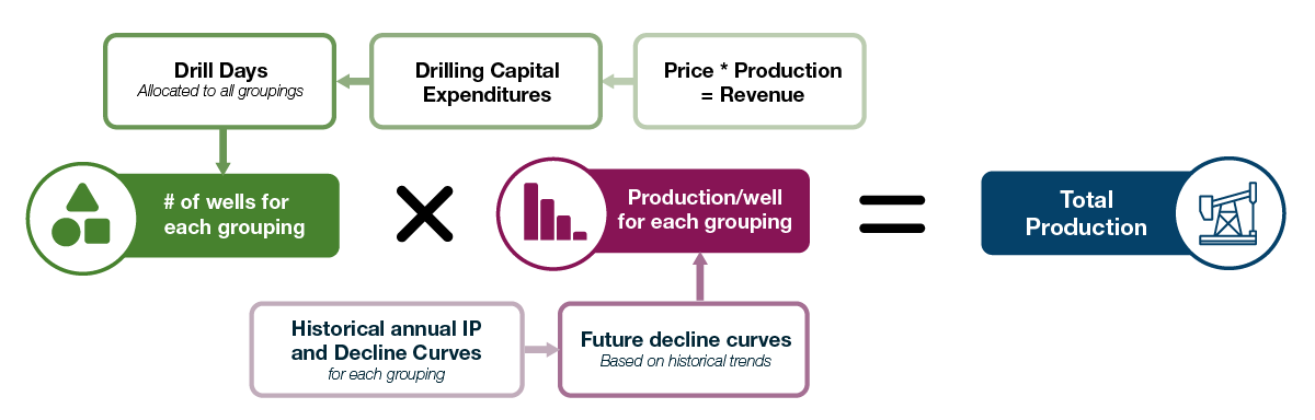
Source and Description
Source: CER
Description: This flowchart illustrates the oil production method. In the top row, there are four steps: 1] calculating revenue based on price multiplied by production, 2] all groupings, and 4] the number of wells drilled per grouping. In the bottom row, there are three steps: 1] collect historical annual initial productivity and decline curves for each grouping, 2] develop future decline curves based on historical trends, and 3] calculate well production profiles for each grouping. Total production is calculated based on the number of wells per grouping (based on the steps in the top row) multiplied by the production per well for each grouping (based on the steps for the bottom row).
Groupings for production decline analysis
To assess oil production for western Canada, oil production and wells are split into various categories as shown in Figure CO.3 Splitting out western Canada by area, class, type, and grouped geological formations results in about 250 total groupings. Of the groupings, approximately 150 have, or have had, producing wells and historical production.
Figure CO.3: Western Canada non-oil sands oil production categories
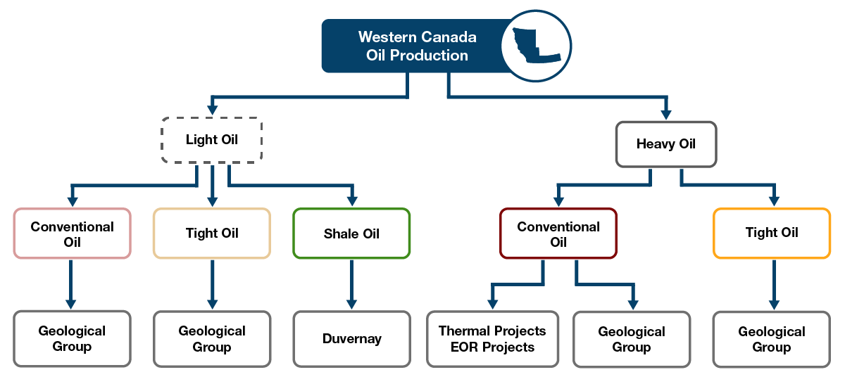
Source and Description
Source: CER
Description: This flow chart shows the categorization of western Canada oil production by class, type, and zone. There are two classes, light oil, and heavy oil. Light oil splits into three types: conventional, tight, and shale oil. The zone for both conventional oil and tight oil is their geological group, while the zone for shale oil is Duvernay. Heavy oil splits into two types: conventional and tight oil. The zone for tight oil is the geological group, while conventional maps to geological group as well as thermal and EOR projects.
Oil Areas
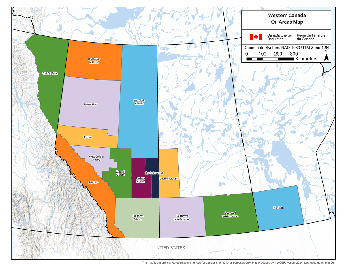
Oil wells and production are grouped geographically based on areasFootnote 3 for Alberta, British Columbia (B.C.), Saskatchewan, and Manitoba (Figure CO.4). The Lloydminster area is further broken down by province. There are 10 areas in Alberta and three in Saskatchewan. Northeast B.C. is considered one area, as is Southwest Manitoba.
Figure CO.4: Western Canada oil areas map
Source and Description
Source: CER
Description: This map shows the oil areas of western Canada used in the model. Wells and production are grouped by area. The map shows oil areas from northeast B.C., Alberta (divided into 10 areas), southern Saskatchewan (divided into 3 areas) and southern Manitoba.
Oil class: light or heavy
Each provincial regulator has its own criteria for classifying crude oil as light, heavy, extra-heavy, or medium. In EF2023, oil production is categorized into only two classes: light and heavy.
Oil Type: conventional, tight, or shale
Once an oil well is classified as light or heavy, it is further categorized as either conventional, tight, or shale.
An oil well is classified as tight if it is a horizontal well that produces from the following formations and was drilled after a certain date:
- Bakken/Three Forks/Torquay: after 2004; MB, SK (Estevan) or AB; Bakken, Torquay and Exshaw Formations
- Beaverhill: after 2008 in AB; Beaverhill Lake Group or Swan Hills Formation (not the Slave Point Formation)
- Belly River: after 2009 in AB; Belly River Group
- Cardium: after 2007 in AB; Cardium Formation
- Charlie Lake: after 2008 in AB; Charlie Lake, Halfway, and Boundary Formations
- Dunvegan: after 2009 in AB; Dunvegan Formation
- Lower Shaunavon: after 2005 in SK, Shaunavon Formation
- Montney/Doig: after 2008 in AB and after 2010 in BC; Montney, Doig, or Triassic Formations
- Pekisko: after 2008 in AB; Pekisko Formation
- Slave Point: after 2008 in AB; Slave Point Formation
- Spearfish: after 2008 in MB; Lower Amaranth Formation
- Viking: after 2007 in SK and AB; Viking Formation
An oil well is considered shale oil if it is horizontal, drilled after 2007, in Alberta and is producing from the Duvernay Formation.
Geologic zone: formation groups
There are thousands of stratigraphic horizons identified in the well data for western Canada. EF2023 analysis aggregates these horizons into broader geologic zones, or groupings of formations. The geologic zones, from shallow/youngest to deeper/oldest are listed in Table CO.1 of this section’s appendix.
- Tertiary
- Upper Cretaceous
- Upper Colorado
- Colorado
- Upper Mannville
- Middle Mannville
- Lower Mannville
- Mannville
- Jurassic
- Upper Triassic
- Lower Triassic
- Triassic
- Permian
- Mississippian
- Upper Devonian
- Middle Devonian
- Lower Devonian
- Siluro/Ordivician
- Cambrian
- PreCambrian
Additional groupings are based on formations of particular importance to production in the Western Canada Sedimentary Basin (WCSB)Definition*, such as the Montney Formation or Duvernay Shale. In addition, oil wells are grouped by the year they were put on production (with all wells prior to 1999 forming a single grouping) so well performance could be analysed over time.
Thermal and enhanced oil recovery (EOR) projects
There are several thermal projects in Saskatchewan’s Lloydminster area, two CO2-EOR projects in Area 14 in Saskatchewan and one in Area 10 in Northwest Alberta. Each of these projects are identified as separate groupings in the analysis. Since these methods of oil extraction are more project based, wells that are identified as part of these projects are not included in the overall decline analysis. Instead, oil production projections for these projects are based on recent production trends, producer plans for continued development, and market assumptions for each scenario projected.
Each of the thermal projects produces heavy, conventional oil from the Mannville Group. The thermal projects are:
- Celtic GP / Sparky
- Lashburn
- Pikes Peak
- Plover Lake
- Sandall Colony
- Bolney
- Dina
- Senlac
- Onion
- Rush Lake
- Dee Valley, Edam Central
- Spruce Lake
The CO2-EOR projects in Saskatchewan produce heavy, conventional oil from the Mississippian zone. The Alberta project produces light, conventional oil from the Mississippian and Devonian zones. The Saskatchewan and Alberta CO2-EOR projects are:
- Weyburn (Area 14)
- Midale (Area 14)
- Zama (Area 10)
New thermal or EOR projects in western Canada would be analysed as individual groupings if developed.
Oil production from gas wells
Oil production from natural gas wells is minimal. In Alberta, less than 2% of conventional and tight oil production comes from gas wells. Since all wells producing oil are included in the existing well analysis, projected oil production from gas wells is embedded in the group projections. Oil production from future gas wells is not directly projected. Analysis of condensate production is included in the natural gas liquids model.
Oil well performance methods
Historical production data is analysed to determine production declines (rates at which production falls over time) which are then used to determine future performance. The analysis includes wells drilled since 2000, which creates a large dataset of historical well production trends. The methods applied to project oil production for existing wells differ from those used to project oil production for future wells.
Historical production data is analysed to determine production declines for each grouping (oil area/class/type/zone/well year) to develop two sets of parameters:
- Group decline parameters: describing production expectations for the entire oil grouping for all wells drilled in each year.
- Average well decline parameters: describing production expectations for the average oil well in the grouping in each year.
The group decline parameters and average well decline parameters resulting from this analysis are available to download as an excel file from the bottom of the EF2023 Data Supplement page. Also included is a dataset of historical monthly oil production, and a dataset of average well production history for each grouping.
The datasets used to estimate group decline parameters are generated by the following: oil production in each grouping is summed to estimate total group oil production (barrels per day (b/d)) by calendar month. Using this dataset, plots of the total daily oil production rate versus total cumulative oil production are generated for each grouping. Oil production in each well is normalized so the first month of production becomes month 1.
Production decline analysis for the average well
For each well year, the daily rate versus cumulative production plot for the average well is evaluated first to establish:
- Initial production rate
- First decline rate
- Second decline rate
- Months to second decline rate – usually around seven months
- Third decline rate
- Months to third decline rate – usually around 25 months
- Fourth decline rate
- Months to fourth decline rate – usually around 45 months
- Fifth decline rate
- Months to fifth decline rate – usually around 90 months
Figure CO.5 shows an example of the plots used to evaluate average well performance, and the different decline rates that are applied to describe the production.
Figure CO.5: Example of a production decline curve for a well
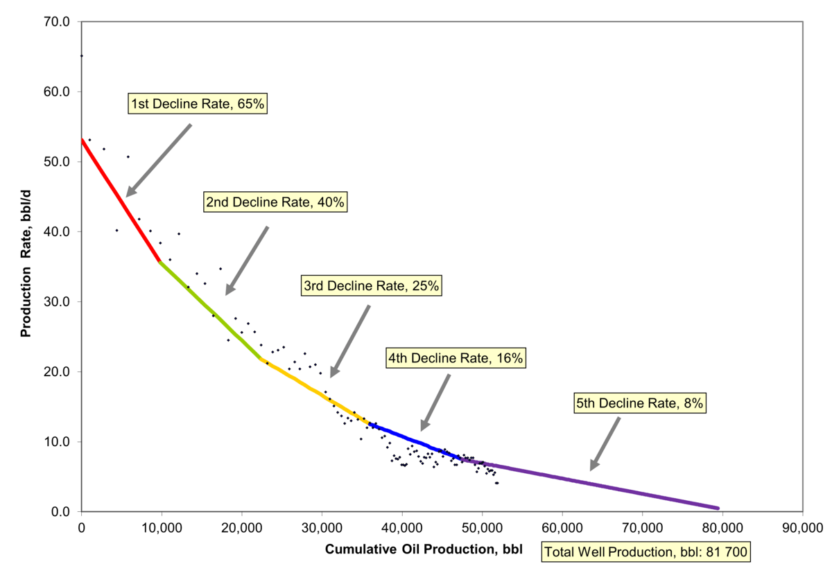
Source and Description
Source: CER, Divestco well data
Description: This chart shows a scatter plot of production rate versus cumulative production, compared against a line chart that is fitted to the points, called a decline curve. The decline curve is broken into five segments based on the decline rate: first decline rate (65%), second decline rate (40%), third decline rate (25%), fourth decline rate (16%), fifth decline rate (8%).
Wells drilled years ago have sufficient data to establish all of the above parameters. However, newer wells have historical production data of shorter duration. Therefore, the projected long-term performance of a newer average well is assumed to be similar to the historical long-term performance of an older average well. In Figure CO.5, the available data is sufficient to determine parameters defining the first, second, third, and fourth decline periods for the well, but the parameters defining the fifth decline period must be assumed based on the analysis of older wells.
Production decline analysis for grouped wells
Performance parameters for an average well are used to calculate the expected group performance. If the data calculated from average well performance data does not provide a good match with the actual historical production data for the group, then the average well parameters may be revised until a good match is obtained between calculated group production data (from average well data) and actual group production data. An example is shown in Figure CO.6.
Figure CO.6: Example of a production decline curve for a group of wells
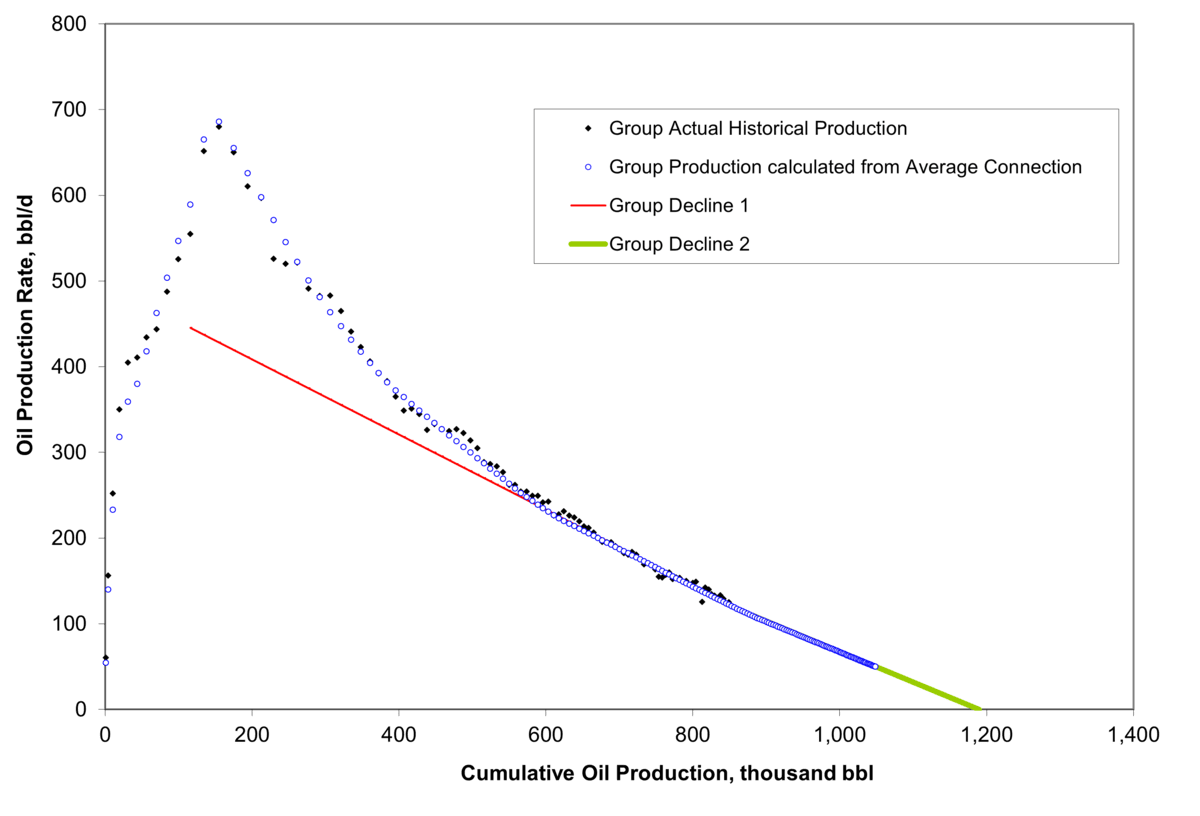
Source and Description
Source: CER, Divestco well data
Description: This chart shows a scatter plot of actual historical production rates over cumulative production for a group of wells. The points are compared against a line that represents the group production decline curve for that group of wells.
The following group performance parameters are determined from the plot of calculated and actual production:
- Production rate at year-end of the previous year
- First decline rate
- Second decline rate (if applicable)
- Months to second decline rate (if applicable)
- Third decline rate (if applicable)
- Months to third decline rate (if applicable)
- Fourth decline rate (if applicable)
- Months to fourth decline rate (if applicable)
- Fifth decline rate (if applicable)
- Months to fifth decline rate (if applicable)
Methods for existing wells
“Existing wells” are those brought on production up to the year the latest well data is available. Group decline parameters are used to project oil production for existing wells.
In groupings of older wells (2001, 2002, etc.), actual group production from recent years is usually stabilized or is near the terminal decline rate established by the pre-1999 aggregate grouping. In these cases, a single decline rate sufficiently describes the entire remaining productive life of the grouping, and the expected performance of the calculated average well has little influence over determination of the group parameters.
In groupings of wells drilled more recently, actual group production history data is unlikely to provide a good basis upon which to project future oil production. In these cases, the expected performance of the average well is more speculative with respect to the applicable current and future decline rates, and older wells group parameters are used as proxy to estimate future decline rates of the recently drilled wells.
Methods for future wells
Future wells are those brought on production for the year the well data ends and onwards. For future wells, projected oil production is based on the number of future wells to be drilled and the expected average performance characteristics of those wells.
The performance of future wells is obtained for each oil grouping by extrapolating the production performance trends for average wells in past years, namely initial productivity of the average well and its associated decline rates, considering technological trends and possible recovery constraints. The parameters of future wells may differ between scenarios, if applicable. Figure CO.7 shows an example of expected initial production rates for an average well for a grouping using historical trends.
Figure CO.7: Example of initial productivity of an average well by year
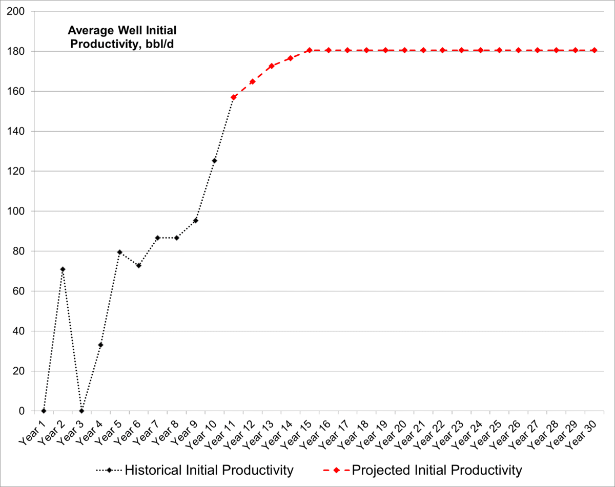
Source and Description
Source: CER, and Divestco well data
Description: This line chart shows an example of initial productivity of an average well by year. It shows historical initial productivity data from year 1 to 10, and then projected initial productivity from year 11 to 30.
The key decline parameters for near-term production projections are the first decline rate, second decline rate, and the months elapsed to reach the second decline rate. Figure CO.8 shows the historical (over the first ten years) and projected values (after year ten) of these parameters for a grouping, and that trend in past well years is used to establish parameters for future years.
Figure CO.8: Example of key decline parameters for an average well over time
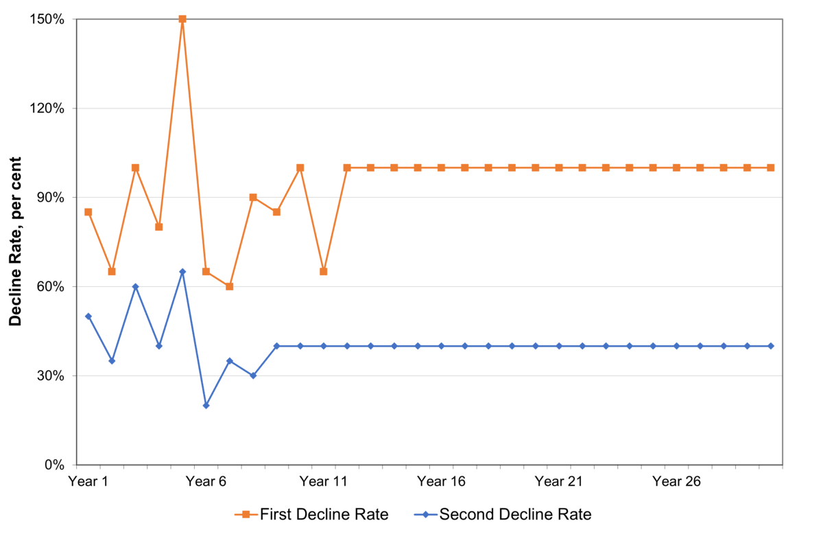
Source and Description
Source: CER, and Divestco well data
Description: This line chart shows an example of first and second decline rates over time. The top line refers to the first decline rate, the bottom line refers to the second decline rate. Both lines show historical values for years 1 to 10, and projected values from years 11 to 30. The lines demonstrate how historical data informs the projections.
Projection of the number of oil wells
Projecting the number of future wells requires an estimate of the annual number of oil wells to be drilled and placed into production for each grouping. Figure CO.2 illustrates the method for production projections. Production for a year is simply the sum of production expected for all wells. The lower pink squares represent the method to get the production per well, by using decline curves as discussed previously. The upper green squares represent the method to get the number of wells drilled in a year.
Gross revenue
The starting point is to calculate gross revenue for a year, which is production multiplied by the assumed price. Gross revenue is then adjusted down by any emission reduction costs. For conventional oil production, the carbon emissions emitted by oil production activities are calculated for the year, and that volume is multiplied by the carbon price for that year. The emission volumes are calculated using the assumed carbon intensity (tonnes of CO2 produced per barrel of oil production) for that year. Historical carbon intensities use available data, and projected carbon intensities for a scenario depend on that scenario’s assumptions regarding mitigation and reduction technologies and measures. The carbon price used in the calculations for a year may include output-based adjustments, which would be representative of the applicable policies in place, in that scenario.
Oil well drill days
A percent of the net revenue (gross revenue less carbon costs) is then assumed to be re-invested back into the industry to drill more wells. This is the drilling capital expenditures for the year. The re-investment percentage for a year is based on trends of previous re-investment ratios and oil prices, and any applicable assumptions for each scenario.
The amount re-invested is divided by the cost per drill day for that year to get total drill days available. Drill day cost for a year is based on historical drill day costs and assumed inflation or deflation rates for the scenario.
Total oil drill days are allocated between each of the oil groupings. The allocation fractions are determined from historical trends and the projection of development potential for each of the groupings. Tables of the historical data (drill days and allocation fractions) and the projected allocation fractions are available to download as an excel file from the bottom of the EF2023 Data Supplement page.
Number of oil wells
The number of oil wells drilled in each year for a grouping is calculated by dividing the drill days allocated to that grouping by the average number of drill days per well. The average number of days to drill a well in a year for a grouping is based on historical trends and any scenario assumptions around efficiency gains or losses, and technological changes.
Once the number of wells per grouping is determined for the year, the monthly distribution of wells drilled over a year is used to determine how many wells are drilled each month for the year. Typically, in western Canada the bulk of drilling occurs in the fall and winter months. In spring the frozen ground thaws, making the ground soft and making it difficult to move materials to drill new wells. Once the ground dries out, activity picks up. This seasonal trend is captured in the analysis through monthly drilling and production calculations.
Production methods
Production projection for a year
With an outlook of the wells drilled per month for a year for each grouping, production for all wells by grouping is simply the expected monthly production rates for a well, via the decline curve parameters, multiplied by the number of wells. This total is production from new wells. Production from wells drilled previously is then calculated and added for the year using decline parameters. Then, monthly production for each grouping is added together to get monthly production for western Canada for that year.
Production projection for all projected years
Production calculated for a year feeds into the gross revenue (production multiplied by price) for the next year, and the process of calculating wells drilled via revenue and production from wells via decline parameters begins again. This way, production from previous years feeds into production for future years, and factors that affect production, like continued low oil prices, higher carbon costs, etc. will have cumulative effects on production over time.
Newfoundland and Labrador offshore oil production
Newfoundland and Labrador offshore oil production has historically come from five major fields: Hebron, Hibernia, North Amethyst, Terra Nova, and White Rose. Total production is calculated on a field-by-field basis based on company reports and data provided by the Canada-Newfoundland & Labrador Offshore Petroleum Board. Fields which are currently producing, or have produced in the past, are categorized as existing fields and their production profile is determined by the time it would take for a field to produce its remaining reserves. Production from offshore fields tends to peak early in their life before tailing off as they mature. Fields that have previously produced, but are currently inactive, can be reactivated based on publicly available information. Production can also be added to existing fields in future time periods based on announcements from operators. New offshore oil fields are uncommon but can be added to the projections when there are strong indicators development will go ahead when considered against other assumptions in the scenario, such as oil prices.
Future production from a project is contingent on whether the project is profitable under the assumptions in each case. To determine if a project will be profitable in our projections, the production cost of each project is assessed on a per barrel basis and compared to the relevant benchmark oil price in each scenario. The cost of production includes capital, operating, and emissions reduction costs. If the cost of production is below the benchmark oil price, the project is deemed to be profitable and will continue to produce oil until its reserves are depleted. If the cost of production for a project is higher than the benchmark price for several years in a row the project is determined to be uneconomic. Uneconomic projects have their production shut in early, and any remaining reserves will not be produced.
Table CO.1: Formation Index
| Formation | Abbreviation | Group Number |
|---|---|---|
| Tertiary | Tert | 2 |
| Upper Cretaceous | UprCret | 3 |
| Upper Colorado | UprCol | 4 |
| Colorado | Colr | 5 |
| Upper Mannville | UprMnvl | 6 |
| Middle Mannville | MdlMnvl | 7 |
| Lower Mannville | LwrMnvl | 8 |
| Mannville | Mnvl | 6;7;8 |
| Jurassic | Jur | 9 |
| Upper Triassic | UprTri | 10 |
| Lower Triassic | LwrTri | 11 |
| Triassic | Tri | 10;11 |
| Permian | Perm | 12 |
| Mississippian | Miss | 13 |
| Upper Devonian | UprDvn | 14 |
| Middle Devonian | MdlDvn | 15 |
| Lower Devonian | LwrDvn | 16 |
| Siluro/Ordivician | Sil | 17 |
| Cambrian | Camb | 18 |
| PreCambrian | PreCamb | 19 |
- Date modified: