
Electricity Supply Model
Model Description
The Electricity Supply Model (ESM) of the Energy Futures Modelling System simulates how the future electricity demand of different economic sectors is satisfied by a combination of electricity generating units and delivery systems. To provide a robust projection of Canada’s electricity supply, the ESM is designed to simulate the typical operations of electric power systems. It models the electricity generating and storage units (including their technical constraints), electricity transmission infrastructure, resource availability, electricity demand, and applicable regulations.
Figure E.1: Electricity Supply Model (ESM) overview

Source and Description
Source: CER
Description: This infographic illustrates how the Electricity Supply Model (ESM) works. The goal of the model is to find the most efficient and cost-effective way to meet electricity demand in each region. The model finds the optimal fuel mix in a given year to meet demand, including costs and emissions. It also finds the best new generating unit type mix for each province or territory’s needs. A map of Canada displays inter-provincial and international transmission lines. The lines are connected to regions comprising of population and generating units.
The ESM projects future electricity infrastructure additions. It also captures potential new net-zero contributions such as hydrogen production and carbon removal, that support Canada’s path to decarbonize. The ESM is built on PyPSA-Can, a Canadian implementation of the Python for Power Systems Analysis package. Figure E.2 shows the main interactions of ESM with other models in the Energy Futures Modelling System. The ESM interacts with other models to obtain the information required to model the electricity system (e.g., electricity demand) and to provide information needed by the other models (e.g., electricity prices).
Figure E.2: Interactions of the Electricity Supply Model with the Energy Futures Modelling System
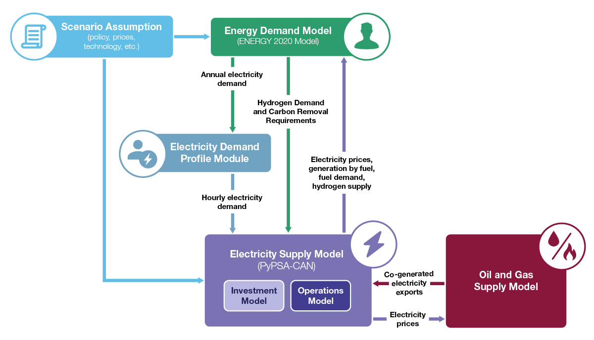
Source and Description
Source: CER
Description: This flow chart illustrates the interactions between the Electricity Supply Model and other models in the Energy Futures Modeling System. The box in the top left corner represents scenario assumptions such as price, policy, and technology parameters. These assumptions influence both the Energy Demand Model and the Electricity Supply Model. The Energy Demand Model provides the Electricity Supply Model with electricity demand and other relevant demands, such as hydrogen produced by electrolysis, and electricity for carbon removal. The Electricity Supply Model provides the energy demand model with electricity prices and other parameters. The Electricity Supply Model also communicates with the oil and gas production models, providing them prices and receiving cogeneration outputs, as required.
Electricity demand profile module
Electricity demand is not constant, it varies over time. The variation is observed across all time periods, including hourly, daily, monthly, and yearly. The factors that lead to variations in electricity demand include weather conditions (e.g., temperature, humidity, etc.), demographic and economic factors of the economy (e.g., types of industries, population density), and consumer behaviour. These variations will be amplified with higher electrification of end-use demands. For example, electrification of space heating will increase the variation of electricity demand due to temperature changes. Electric vehicle charging will add new end-user demands.
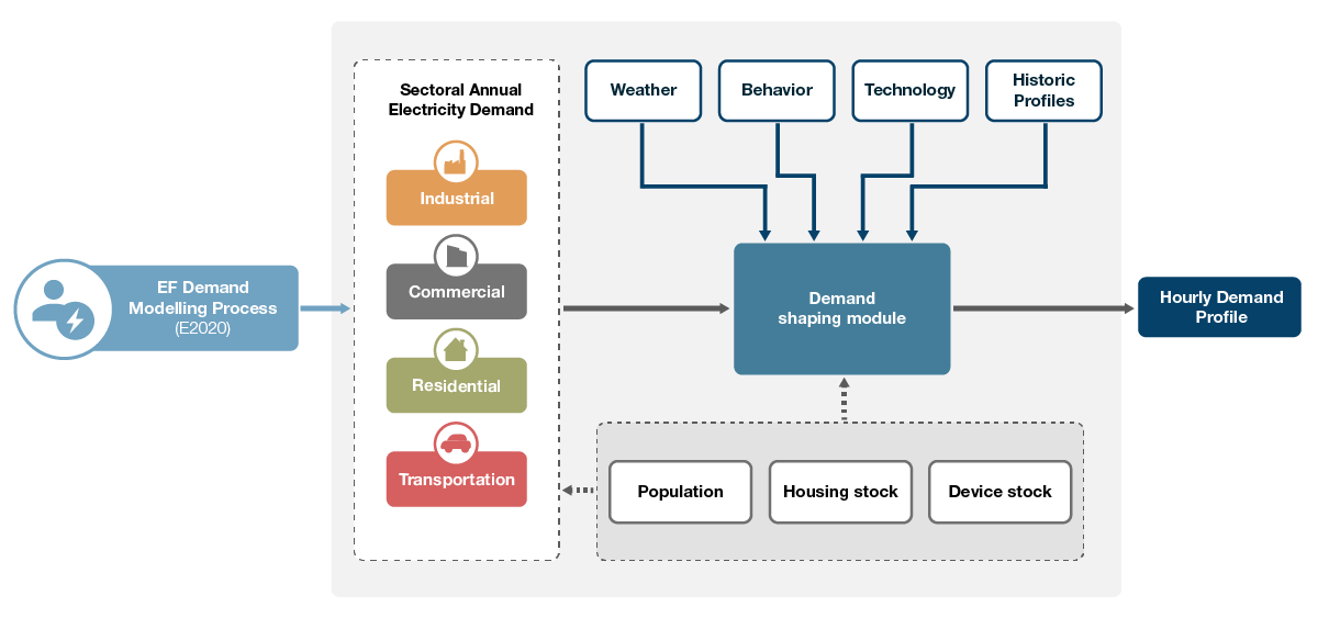
The Energy Demand Model, ENERGY 2020, produces provincial and territorial electricity demand projections at annual time scales. The Electricity Demand Profile module converts the annual projections into hourly electricity demand profiles covering all analysis years in the outlook. The process is illustrated in Figure E.3.
The demand shaping module splits annual electricity demand into hourly intervals based on a variety of sources including: temperature data consistent with the solar resource data used in PyPSA-Can, hourly load shapes for the United States (U.S.) by end-use from the National Renewable Energy Laboratory Electrification Futures study, and various academic and institutional studies.
Figure E.3: Electricity demand profile module
Source and Description
Source: CER
Description: This flow chart describes the electricity demand profile module. This module converts annual electricity demands from the Energy Demand Model and converts them into electricity demand in all 8,760 hours in each year of the projection period, for various sectors and end-uses. The load profiles are influenced by a variety of factors including weather, technology, behaviour assumptions, and historic profiles.
Electricity supply module
At the center of the ESM are the electricity system operations simulation model and infrastructure investment planning model. The operations simulation model considers the hourly demand projections of Canadian provinces and territories produced by the Electricity Demand Profile module. The operations model then determines which electricity generating units and other supply resources are used to satisfy demand at any given hour using a combination of available supply resources:
- Consider the production capacity of generating units in that region to meet that demand in that hour. The available capacity is generally limited by the combined capacity of all generating units installed at a given time. However, in the case of variable generating units (e.g., wind, solar, and run-of-the-river hydro units), the power generation capacity at a given time is limited by the resource availability (e.g., wind speed and intensity of solar resources).
- The full, or partial electricity demand, in a given region can be met by electricity exported from a neighbouring region if sufficient electricity transmission capacity is available.
- Electricity storage units with sufficient stored energy, could be used to meet demand in a given region.
Electricity operations model
The operating model will deploy the electricity supply resources up to their available potential in ascending order of operating cost until the demand is met. The operating cost of electricity supply resources depends on corresponding fuel prices, variable operating costs, operating efficiencies (i.e., the amount of fuel required to produce a unit of electricity), and in some cases, applicable carbon prices.
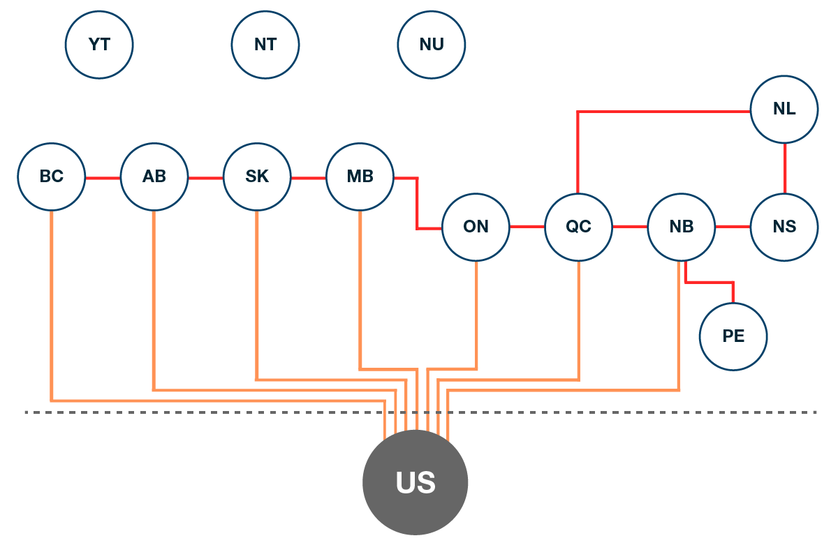
Figure E.4: Regional representation of the ESM and main transmission lines
Source and Description
Source: CER
Description: This figure illustrates the regional connections of the Electricity Supply Model and main transmission lines. Each circle represents a province, and the U.S. Lines that connect circles represent major transmission lines. The three territories are not connected to other regions via a transmission line.
Some hundreds of electricity-generating units that use different technologies and fuels are installed in different parts of the provinces and territories. Those generating units are connected to electricity end users by transmission and distribution lines. In the ESM, the electricity transmission system is represented in a limited capacity. The ESM tracks all inter-provincial electricity transmission lines. However, currently, the transmission lines within a given province are not modelled. The costs associated with delivering electricity to the consumers through intra-provincial transmission lines are exogenously estimated. Figure E.4 shows the main transmission lines tracked by the ESM.
The ESM tracks electricity generation and storage units installed in each province. The demand in each of those regions is satisfied by the electricity supply resources in the region or neighbouring regions linked by transmission lines. The ESM also tracks electricity imports and exports with the U.S.
Demand and infrastructure needs
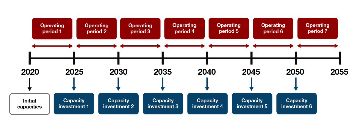
The operations model determines the supply resources used to meet electricity demand throughout the outlook period. As existing supply resources retire and electricity demand grows, new electricity infrastructure needs to be added. The investment planning model considers the electricity demand projections in a given region and adds electricity generation, storage, and transmission infrastructure as required. The current model adds infrastructure investments in five-year intervals (Figure E.5) within the outlook period. To add infrastructure, the investment model considers possible new infrastructure and adds the ones with the minimum initial cost (i.e., capital cost) and operating cost over the outlook period.
Figure E.5: Electricity sector investments and operations
Source and Description
Source: CER
Description: This timeline graphic shows the operating and investment dynamics in the Electricity Supply Model. Investments begin with initial capacities in 2020 and investments are optimized every five years after. Between these periods there are operating periods where the model supplies the annual hourly loads using the available generation, storage, and transmission systems.
The current model considers all existing generating units installed in Canadian provinces. The information about the current units is obtained from different sources, including Statistics Canada and the different utilities that operate them in their respective provinces. Table E.1 lists the new electricity generation and storage technologies that are considered to be built over the outlook period, along with current cost and performance estimates.Footnote 1 Currently, the model only considers increasing the capacities of transmission lines among Canadian provinces, as shown in Figure E.4. New transmission lines between Canadian provinces and the U.S. are not considered in the model, assuming that no new incremental power lines are added.
Other model features
In addition to simulating the supply of electricity to end-use customers, the ESM tracks some new applications of electricity as well as the overall contribution of the electricity sector to achieve net-zero emissions.
Hydrogen production
One of the new applications is hydrogen production using electrolysis. The model considers the demand for electrolysis hydrogen and operates electrolyzers to satisfy the demand. Since hydrogen can be stored, the time in which hydrogen could be produced is flexible. Therefore, the electricity operations model decides the hours in which the electrolyzers are operated so that the operating costs would be minimized. For example, if a higher amount of variable renewable-powered electricity is available during periods of low electricity demand, the excess electricity could be used to produce hydrogen.
Table E.1: Electricity generation and storage technologies with current costs and heat rates
| Technology | Overnight capital cost ($/kW) | Variable O&M Cost ($/kWh) | Fixed O&M Cost ($/kW-yr) | Heat rate (MMbtu /MWh) |
|---|---|---|---|---|
| Renewable generation | ||||
| Offshore wind | 3561 | 0.0 | 189 | 3.4 |
| Onshore wind | 1900 | 0.0 | 72 | 3.4 |
| Solar P.V. utility scale | 1700 | 0.0 | 39 | 3.4 |
| Distributed solar P.V. – commercial | 2250 | 0.0 | 30 | 3.4 |
| Distributed solar P.V. – residential | 3450 | 0.0 | 45 | 3.4 |
| Geothermal | 7100 | 1.0 | 137 | 22.7 |
| Biomass – steam cycle | 5875 | 7.0 | 200 | 11.0 |
| Biomass – IGCC | 6071 | 13.0 | 220 | 9.6 |
| Biopower IGCC + CCS | 9223 | 19.0 | 270 | 9.7 |
| Waste steam cycle | 6463 | 7.7 | 220 | 13.3 |
| Waste LFG or A.D. in ICE | 4765 | 9.0 | 112 | 14.8 |
| Hydropower large dam >100 MW | 4500 | 0.0 | 51 | 4.0 |
| Hydropower small dam <100 MW | 6150 | 0.0 | 82 | 4.0 |
| Hydropower repurposing other dams | 4200 | 0.0 | 66 | 4.0 |
| Hydropower run-of river <10 MW | 5025 | 0.0 | 58 | 4.0 |
| Hydropower run-of river 10-100 MW | 3910 | 0.0 | 45 | 4.0 |
| Hydropower run-of river >100 MW | 3100 | 0.0 | 36 | 4.0 |
| Hydropower redevelopment | 3100 | 0.0 | 82 | 4.0 |
| Tidal | 15341 | 0.0 | 150 | 4.0 |
| Wave | 10500 | 0.0 | 131 | 22.7 |
| Hydrogen fired generation | ||||
| Hydrogen SOFC fuel cell | 6850 | 0.6 | 48 | 6.5 |
| Hydrogen steam cycle | 1575 | 10.0 | 39 | 9.9 |
| Hydrogen combined cycle | 1775 | 10.0 | 52 | 6.5 |
| Blended hydrogen CC + CCS | 3300 | 12.0 | 112 | 6.8 |
| Nuclear energy-based generation | ||||
| Nuclear – small modular reactor | 9262 | 3.0 | 63 | 10.5 |
| Nuclear – conventional | 9100 | 4.0 | 242 | 8.4 |
| Fossil fuel fired generation | ||||
| Natural gas – simple cycle | 1300 | 9.0 | 38 | 9.7 |
| Natural gas – simple cycle with CCS | 4746 | 10.0 | 130 | 10.9 |
| Natural gas combined cycle | 1450 | 9.0 | 50 | 6.4 |
| Natural gas combined cycle with CCS | 3705 | 10.0 | 110 | 7.2 |
| Coal advanced supercritical SC | 3075 | 11.0 | 52 | 8.5 |
| Coal SC + CCS | 5535 | 22.0 | 99 | 9.3 |
| Electricity storage | ||||
| Hydrogen fuel cells with electrolyzers | 4849 | 0.6 | 38 | 8.1 |
| Compressed air energy storage | 1989 | 2.0 | 18 | 10.5 |
| Lithium battery storage | 435 | 0.0 | 65 | 4.0 |
| Pumped hydro storage | 2300 | 0.7 | 45 | 4.3 |
Carbon removal
Another new application tracked by the ESM is the operation of direct air capture (DAC) units. DAC is a technology that can be used to remove carbon dioxide from the atmosphere. A significant amount of electricity and thermal energy is required to operate DAC. Like electrolyzers, the exact operational time of DAC is flexible. Therefore, the operations model of the ESM would operate DAC in a way that the total operating cost of the electricity system is minimalized.
Co-generated electricity
Some industrial facilities in Canada operate cogeneration units, which involve the concurrent production of electricity or mechanical power and useful thermal energy (heating and/or cooling) from a single source of energy. In some cases, the electricity produced by the cogeneration units is more than the electricity demand of the host facility. The excess electricity could be exported to the grid. Most cogeneration units are observed in the oil sands sector of Alberta. Therefore, the ESM interacts with the Oil & Gas Supply model to track available co-generated electricity (see Figure E.2).
Main data and assumptions
Technology cost and performance data
The criteria used to build and operate electricity infrastructure in the model is minimizing the initial and operating costs. Therefore, the ESM requires information on the costs and performance of electricity generation units, storage units, and transmission systems. The transmission system cost information is extracted from publicly available sources as well as from project-specific information. For generation and storage units, the model considers factors from two cost categories:
- Initial investment cost
- The initial cost of generation/storage equipment
- Project development cost
- Cost of new transmission required to connect generation/storage units into the transmission system
- Costs incurred at the point of interconnection
- Operations costs
- Fixed operating and maintenance cost
- Fuel cost
- Non-fuel operating costs
- Cost of carbon emissions
These costs are extracted from expert sources such as the International Energy Agency (IEA), the U.S. National Renewable Energy Laboratory (NREL), and International Renewable Energy Agency (IREA). The cost and performance data are also linked with the main scenario assumptions. For example, in a scenario where Canada and the rest of the world achieve net-zero emissions, it is possible there will be a high level of innovation in low emission technologies, lowering their costs and increasing performance. Similarly, in a scenario with a higher carbon price, the operating cost of technologies with non-zero emissions would be higher. As shown in Figure E.1, the ESM makes scenario-specific assumptions about the costs and performance of electricity generation and storage technologies.
Renewable resource data
Renewable based generation is expected to dominate electricity generation in a net-zero future. The available renewable energy resources (e.g., wind, solar, hydro, biomass) vary across the country. Also, the availability of most renewable resources varies over different time periods. Therefore, the ESM requires reliable estimates of renewable resource availability in Canadian provinces and territories. The model obtains the renewable resource information from reputable sources, including the following:
- Engineering Climate Datasets developed by Environment and Climate Change Canada (ECCC)
- Renewable resource datasets of North America developed by the U.S. National Renewable Energy Laboratory (NREL)
- CER Bioenergy Supply Model resource data
- Geological Survey of Canada
- Various provincial utilities and agencies
Main Model Outputs
The ESM produces the following outputs. The ESM estimates those outputs at hourly intervals, and the values are aggregated to produce annual results:
- Installed electricity generation and storage capacity by technology and region.
- Annual electricity generation by technology and region.
- Inter-provincial transmission capacity by transmission corridor.
- Annual electricity interchanges across provinces and the U.S.
- Average annual cost of electricity generation by region.
- Annual GHG emissions from electricity generation by region.
- Date modified: