
Natural Gas Production Model
Model description
Canadian natural gas production consists of conventionalDefinition*, tightDefinition*, shaleDefinition*, solutionDefinition*, and coalbedDefinition* natural gas production from western Canada and conventional natural gas production from onshore New Brunswick, Ontario, and northern Canada. Western Canadian natural gas production projections include trends in well production characteristics and resource development expectations. Different approaches were used for other regions of Canada where production is sourced from a smaller number of wells.
Natural gas production in EF2023 refers to marketable natural gas production.
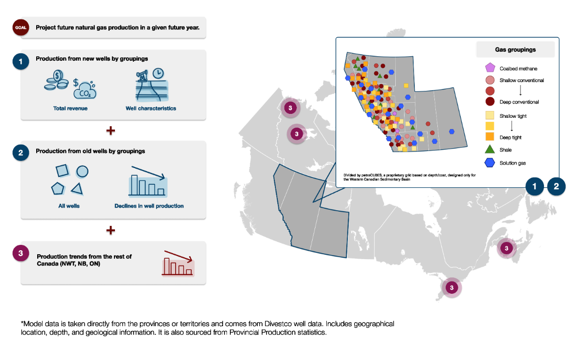
Figure NG.1: Natural gas model overview
Source and Description
Source: CER
Description: The infographic displays an illustrative overview of the model used to determine total Canadian natural production in a given year. The model components include:
- Natural gas production from new wells, including total revenue and well characteristics (like depth and age).
- Natural gas production from old wells by groupings, factoring in all wells and any declines in natural gas production.
- Production trends from the rest of Canada, including the Northwest Territories, New Brunswick, and Ontario.
The infographic also displays natural gas PetroCUBE groupings in western Canada and natural gas production areas in the rest of Canada. The western Canadian natural gas groupings categorize natural gas by area, conventional, tight, shale, coalbed methane, and solution gas types, and by shallow to deep zones.
Western Canada (British Columbia, Alberta, and Saskatchewan)
CER models that project natural gas production estimate the capacity of future production to produce gas. They do not account for possible reductions in actual production due to intermittent weather, natural disasters, equipment failure, or other potential production interruptions. It equals the production capability of wells multiplied by the expected number of wells.
The number of wells drilled in the future in the model depends on investment. Total revenue available to industry in any given year is estimated by applying future prices of gas to total production, minus emissions costs. Some of this revenue is then reinvested as capital expenditures in new wells. The capital expenditures divided by the daily cost of drilling determines the number of drill days available in a year. The number of new wells drilled in each year is equal to the number of drill days per year divided by the number of days required to drill and complete an average well. The projected production of an average well is based on historical performance, specifically on how the initial production (IP) rates and decline rates change over time. Figure NG.2 summarizes the natural gas production projection method.
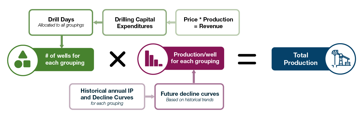
Figure NG.2: Flowchart of the natural gas production method
Source and Description
Source: CER
Description: This flowchart describes the natural gas production method. In the top row, there are four steps: 1] calculating revenue based on price multiplied by production, 2] estimating drilling capital expenditures based on the revenue, 3] calculating drill days allocated to all groupings, and 4] the number of wells drilled per grouping. In the bottom row, there are three steps: 1] collect historical annual initial productivity and decline curves for each grouping, 2] develop future decline curves based on historical trends, and 3] calculate production per well for each grouping. Total production is calculated based on the number of wells per grouping (based on the steps in the top row) multiplied by the production per well for each grouping (based on the steps for the bottom row).
Groupings for production decline analysis
To assess natural gas production for western Canada, natural gas production and wells are split into various categories as shown in Figure NG.3. Gas production from the Montney Formation is separated from the other tight gas sources as it is, and will continue to be, the main focus of activity and production in western Canada.
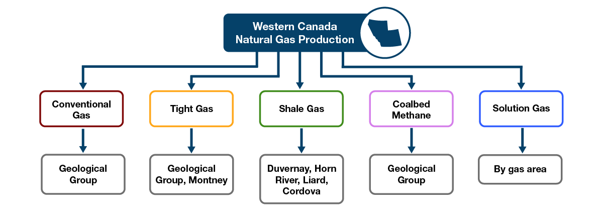
Figure NG.3: Western Canada natural gas production categories
Source and Description
Source: CER
Description: This flow chart shows the categorization of western Canada natural gas production by type and zone. For western Canada natural gas production, there are five types of production, each with a respective zone (in parenthesis): conventional gas (zone: geological group), tight gas (zone: geological group, Montney), shale gas (zone: Duvernay, Horn River, Liard, Cordova), coalbed methane (zone: geological group), and solution gas (zone: by gas area).
Production decline analysis on historical production data was used to determine parameters that define future performance. The method to determine gas production related to oil wells (solution gas) is described below.
Natural gas areas
Natural gas wells and production are grouped geographically based on areasFootnote 1 for Alberta, British Columbia (B.C.), and Saskatchewan, as shown in Figure NG.4.
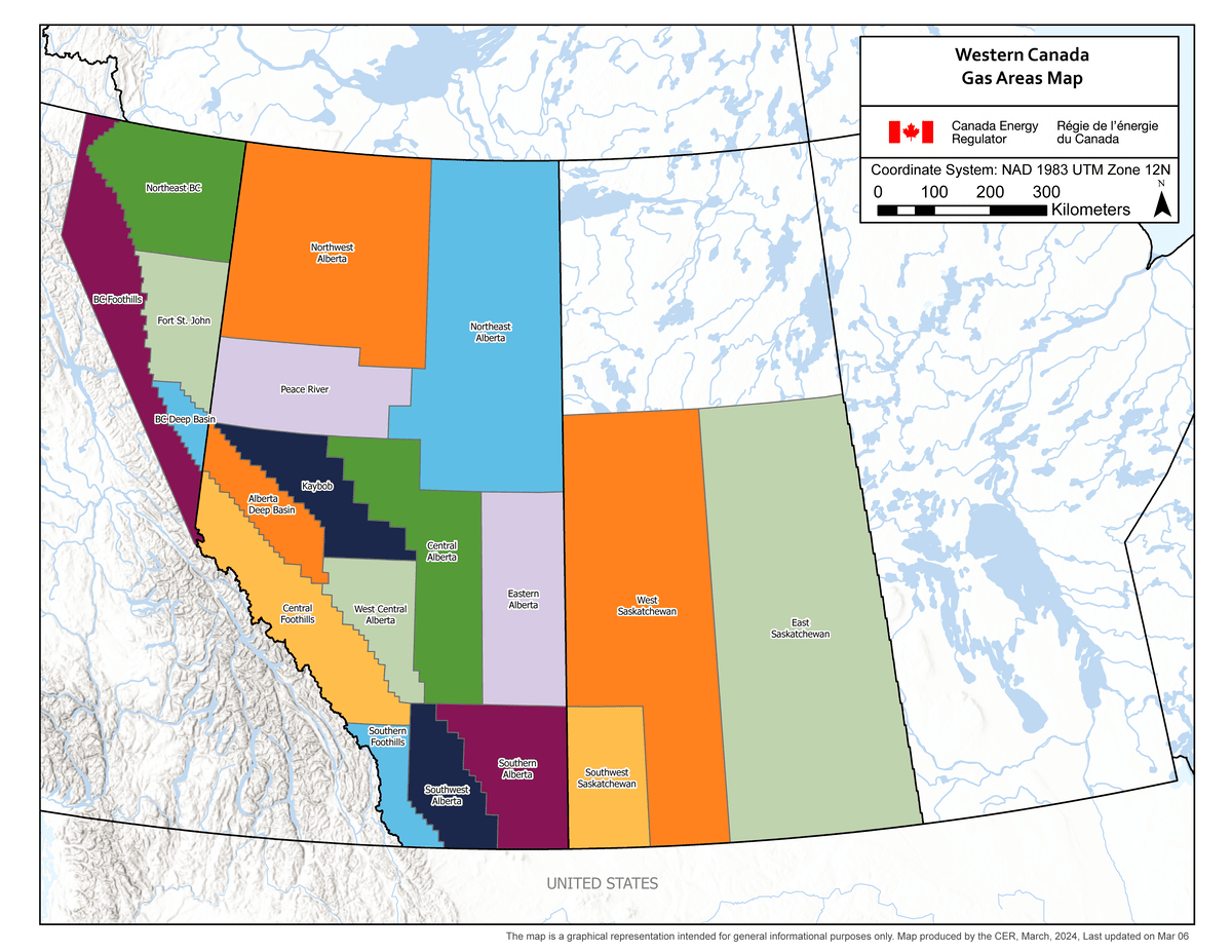
Figure NG.4: Western Canada natural gas areas map
Source and Description
Source: CER
Description: This map shows the natural gas areas of western Canada used in the model. Production is grouped by area. The map shows natural gas areas from northeast British Columbia (B.C.) (divided into 4 areas), Alberta (divided into 12 areas), and Saskatchewan (divided into 3 areas). There is no natural gas production from Manitoba in the model.
Type: conventional, tight, shale, coalbed methane (CBM), or solution gas
Once the area for a natural gas well is assigned, the type of gas from that well is determined. The type of natural gas can either be conventional, tight, shale, coalbed methane (CBM), or solution.
Tight gas
A natural gas well is classified as tight if it is a horizontal well that produces from the following formations and was drilled after a certain date:
- Montney B.C.: in B.C., Montney or Doig Phosphate Pool
- Montney Alberta: after 2004; in Alberta, Montney or Doig, or Triassic Pool and Formation
Shale gas
A natural gas well is classified as shale if it is a horizontal well that produces from the following categories:
- Duvernay: after 2009; in Alberta, Duvernay Pool and Formation
- Cordova: in B.C.; Helmet field/area, Muskwa, Cordova Embayment, Otter Park, Klua, or Evie Pools
- Horn River: in B.C.; Horn River or Horn River Basin field/area
- Liard: Liard or Liard Basin Basin field/area
Coalbed methane gas (CBM)
CBM groupings cover parts of British Columbia and Alberta, and are grouped primarily by zone into three categories:
- Horseshoe Canyon Main Play
- Mannville CBM
- Other CBM
Solution gas
Solution gas is natural gas that is produced along with crude oil from oil wells. The natural gas is associated with oil production and is also commonly referred to as associated gas. Generally, solution gas is gas that is part of oil production and needs to be separated out of the crude oil, and associated gas is natural gas that comes out of the well but is separate from the crude oil and not dissolved into the crude oil. EF2023 classifies all natural gas from oil wells as solution gas for simplicity.
Geological zone: formation groups
There are thousands of stratigraphic horizons identified in the well data for western Canada. This model aggregates these horizons into broader geologic zones, or groupings of formations. The geologic zones are listed in Table NG.1.
These geologic zones may be further aggregated into groupings of specific formations, based on criteria such as the area, similar well characteristics, or number of wells.
The groupings (conventional, tight, shale, CBM, and solution gas resources by area and depth)Footnote 2 in Alberta, B.C., and Saskatchewan, are shown in Figure NG.5. In this analysis, gas production from the Montney Formation is separate from the other tight gas sources and is shown in Figure NG.5 by orange squares marked with an ‘M’. In total, western Canada has about 150 gas resource groupings, each with its own set of monthly production and annual gas compositions.
Figure NG.5: Western Canada natural gas groupings map
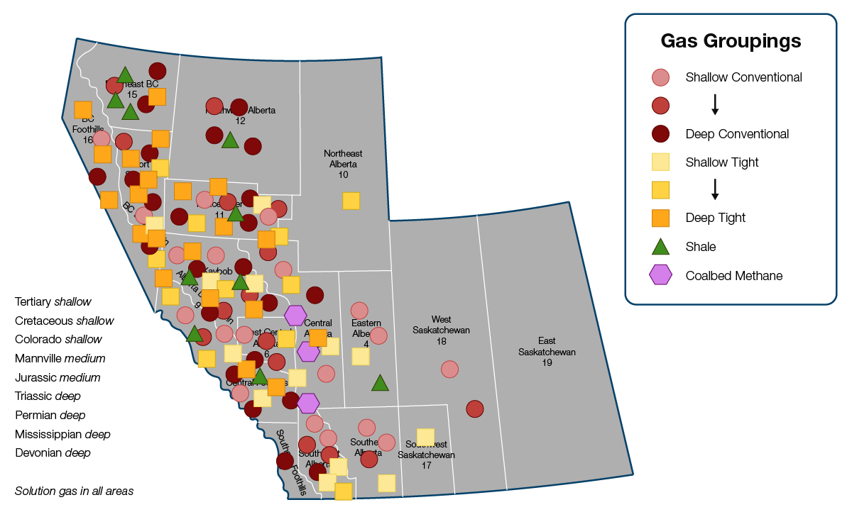
Source and Description
Source: CER
Description: This map shows the natural gas groupings in western Canada. The groupings are categorized by: area (geographic location), conventional, tight, shale, CBM, and solution gas types (by shape and colour); and by shallow to deep zones (lighter to darker for each colour). Each grouping is represented by a shape.
Within each grouping, natural gas wells were grouped by well year, with all wells drilled prior to 1999 forming a single group, and separate yearly classifications for each year from 1999 and on. Thus, for each grouping, average well performance can by analysed over time to see how initial production (IP) rates and declines change as the resource is developed and as technology evolves.
Natural gas well performance methods
Historical production data is analysed to determine production declines, which are then used to determine future performance. The analysis includes wells drilled since 2000, which creates a large dataset of historical well production trends. The methods applied to project natural gas production for existing wells differ from those used to project natural gas production for future wells.
Historical production data is analysed to determine production declines for each grouping (natural gas area/type/zone/well year) to develop two sets of parameters:
- Group decline parameters describe production expectations for the entire grouping for all wells drilled in each year.
- Average well decline parameters describe production expectations for the average natural gas well in the grouping in each year.
The group decline parameters and average well decline parameters resulting from this analysis are available to download as an excel file from the bottom of the EF2023 Data Supplement page.
A dataset of historical monthly natural gas production, and a dataset of average well production history, are created for each grouping.
The datasets used to estimate group decline parameters are generated by the following:
- Natural gas production in each grouping is summed to estimate total group natural gas production in thousands of cubic feet per day (Mcf/d) by calendar month.
- Using this dataset, plots of the total daily natural gas production rate versus total cumulative natural gas production are generated for each grouping.
The datasets used to determine average well decline parameters are generated by the following:
- The historical, monthly natural gas production for each well in the grouping is put in a database.
- For each well, the production months are normalized such that the month the well started producing becomes the first production month.
- The total natural gas production by normalized production month is then divided by the total number of wells in the grouping to determine normalized, monthly natural gas production for the average well.
- The normalized, monthly natural gas production is then divided by the average number of days in a month, or 30.4375 (365.25 divided by 12), to determine the daily production rates for the average well in the grouping.
- Using this dataset, plots of the daily natural gas production rate versus cumulative natural gas production for the average well are generated for each grouping.
After the average well’s historical production for each grouping and year is determined, each average well is evaluated in sequence, from 2000 through to the latest year well data is available.
Production decline analysis for the average well
For each well year, the daily rate versus cumulative production plot for the average well is evaluated first to establish:
- Initial production rate
- First decline rate
- Second decline rate
- Months to second decline rate (usually around seven months)
- Third decline rate
- Months to third decline rate (usually around 25 months)
- Fourth decline rate
- Months to fourth decline rate (usually around 45 months)
- Fifth decline rate
- Months to fifth decline rate – usually around 90 months
Figure NG.6 shows an example of the plots used to evaluate average well performance, and the different decline rates that are applied to describe the production.
Figure NG.6: Example of a production decline curve for a well
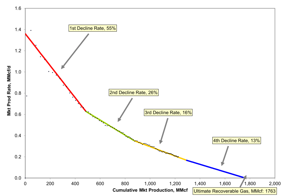
Source and Description
Source: CER and Divestco well dataCER
Description: This chart shows a scatter plot of production rate versus cumulative production, compared against a line chart that is fitted to the points, called a decline curve. The decline curve is broken into four segments based on the decline rate: first decline rate (55%), second decline rate (26%), third decline rate (16%), and fourth decline rate (13%).
Wells drilled years ago have sufficient data to establish all of the above parameters. However, newer wells have historical production data of shorter duration. Therefore, the projected long-term performance of a newer average well is assumed to be similar to the historical long-term performance of an older average well. In Figure NG.6, the available data is sufficient to determine parameters defining the first, second, and third decline periods for the well, but the parameters defining the fourth and fifth decline periods must be assumed based on the analysis of older wells.
Production decline analysis for the group data
Performance parameters for an average well are used to calculate the expected group performance. If the data calculated from average well performance data does not provide a good match with the actual historical production data for the group, then the average well parameters may be revised until a good match is obtained between calculated group production data (from average well data) and actual group production data. An example is shown in Figure NG.7.
Figure NG.7: Example of a production decline curve for a group of wells
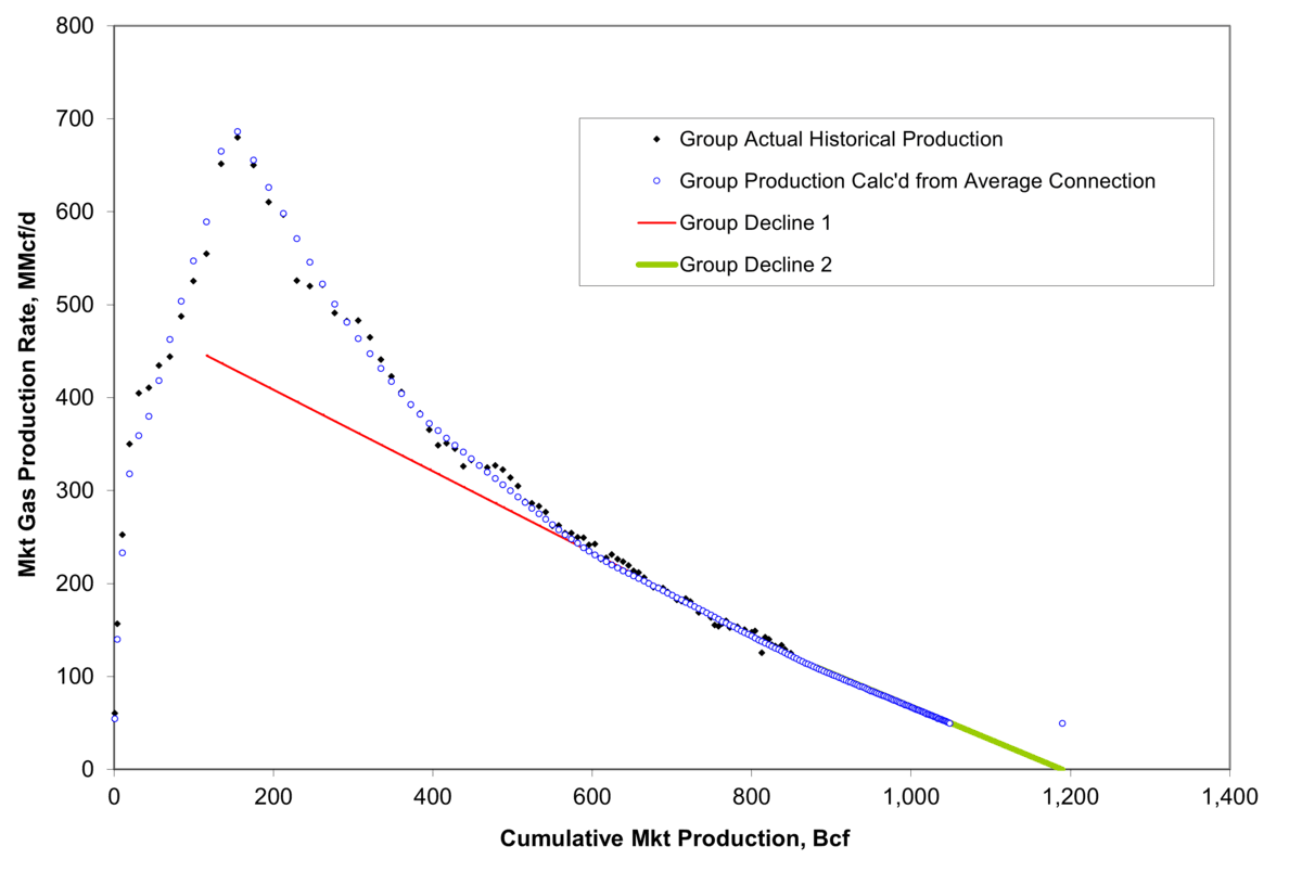
Source and Description
Source: CER and Divestco well data
Description: This chart shows a scatter plot of actual historical production of a group of wells calculated from average connection. The points reflect the marketable gas production rate against cumulative marketable gas production. The points are compared against a line that represents the group production decline curve for a group of wells.
The following group performance parameters are determined from the plot of calculated and actual production:
- Production rate at year-end of the previous year
- First decline rate
- Second decline rate (if applicable)
- Months to second decline rate (if applicable)
- Third decline rate (if applicable)
- Months to third decline rate (if applicable)
- Fourth decline rate (if applicable)
- Months to fourth decline rate (if applicable)
The production decline analysis procedure described above is also applied to the CBM groupings and shale gas. Mannville CBM connections have a different performance profile than the other gas resources in the WCSBDefinition*. While gas wells for all other groupings can be described by an initial production rate that declines in a relatively predictable manner, Mannville CBM connections go through a dewatering phase (removing water) with gas production increasing over a period of months to a peak rate. After the peak rate is reached, decline will occur. Thus, a slightly different set of parameters is used to describe performance of the average well for Mannville CBM, with initial production rate being replaced by “months to peak production” and “peak production rate”.
Methods for existing wells
“Existing wells” are those that started production up to the year the latest well data is available. Group decline parameters are used to project natural gas production for existing wells.
In groupings of older wells (2001, 2002, etc.), actual group production from recent years is usually stabilized or is near the terminal decline rate established by the pre-1999 aggregate grouping. In these cases, a single decline rate sufficiently describes the entire remaining productive life of the grouping, and the expected performance of the calculated average well has little influence over determination of the group parameters.
In groupings of wells drilled more recently, actual group production history data is unlikely to provide a good basis upon which to project future natural gas production. In these cases, the expected performance of the average well is more speculative with respect to the applicable current and future decline rates, and older wells’ group parameters are used as proxy to estimate future decline rates of the recently drilled wells.
Methods for future wells
Future wells are those brought on production for the year the well data ends and onwards. For future wells, projected natural gas production is based on the number of future wells to be drilled and the expected average performance characteristics of those wells.
The performance of future wells is obtained for each natural gas grouping by extrapolating the production performance trends for average wells in past years, namely initial productivity of the average well and its associated decline rates, considering technological trends and possible recovery constraints. The parameters of future wells may differ between scenarios, if applicable. Figure NG.8 shows an example of expected initial production rates for an average well for a grouping using historical trends.
Figure NG.8: Example of initial productivity of an average well by year
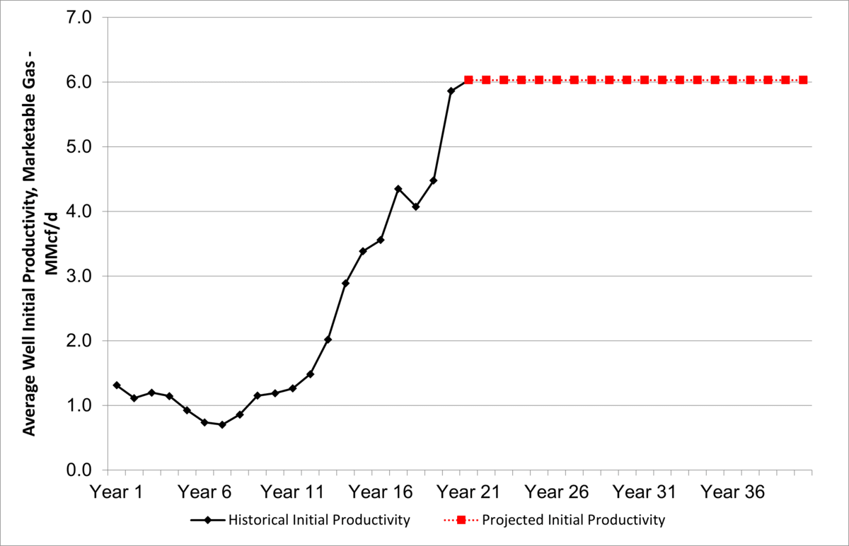
Source and Description
Source: CER and Divestco well data
Description: This line chart shows an example of initial productivity of an average well by year. It shows historical initial productivity data from year 1 to 20, and then projected initial productivity from year 21 to 40.
The key decline parameters for near-term production projections are the first decline rate, second decline rate, and the months elapsed to reach the second decline rate. Figure NG.9 shows the historical and projected values of these parameters for a grouping, and that trends in past well years are used to establish parameters for future years.
Figure NG.9: Example of key decline parameters for an average well over time
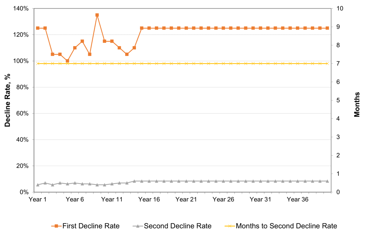
Source and Description
Source: CER and Divestco well data
Description: This line chart shows an example of first and second decline rates for a grouping. The top line refers to the first decline rates, the bottom line refers to second decline rates. The line in the middle shows the months from first to second decline rate (which in this case is 7, on the right axis). Both lines show historical values for years 1 to 10, and projected values from years 11 to 40. The lines demonstrate how historical data informs the projections.
Projection of the number of natural gas wells
Projecting the number of future wells requires an estimate of the annual number of natural wells to be drilled and placed into production for each grouping. Figure NG.2 illustrates the method for production projections. Production for a year is simply the sum of production expected for all wells. The lower pink squares represent the method to get the production per well, by using decline curves as discussed previously. The upper green squares represent the method to get the number of wells drilled in a year.
Gross revenue
The starting point is to calculate gross revenue for a year, which is production multiplied by the assumed price. Gross revenue is then adjusted down by any emission reduction costs. For natural gas production, the carbon emissions emitted by natural gas production activities are calculated for the year, and that volume is multiplied by the carbon price for that year. The emission volumes are calculated using the assumed carbon intensity (tonnes of CO2 produced per thousand cubic feet of natural gas production) for that year. Historical carbon intensities use available data, and projected carbon intensities for a scenario depend on that scenario’s assumptions regarding mitigation and reduction technologies and measures. The carbon price used in the calculations for a year may include output-based adjustments, which would be representative of the applicable policies in place in that scenario.
Drill days
A percent of the net revenue (gross revenue less carbon costs) is then assumed to be re-invested back into the industry to drill more wells. This total is the drilling capital expenditures for the year. The re-investment percentage for a year is based on trends of previous re-investment ratios and natural gas prices, and any applicable assumptions for each scenario.
The amount re-invested is divided by the cost per drill day that year to get total drill days available. Drill day cost for a year is based on historical drill day costs, assumed inflation or deflation rates, and any technological changes assumed for the scenario.
Total natural gas drill days are allocated between each of the natural gas groupings. The allocation fractions are determined from historical trends and the projection of development potential for each of the groupings. Tables of the historical data (drill days and allocation fractions) and the projected allocation fractions are are available to download as an excel file from the bottom of the EF2023 Data Supplement page.
Natural gas wells
The number of natural gas wells drilled in each year for a grouping is calculated by dividing the drill days allocated to that grouping by the average number of drill days per well. The average number of days to drill a well in a year for a grouping is based on historical trends and any scenario assumptions around efficiency gains or losses.
Once the number of wells per grouping is determined for the year, the monthly distribution of wells drilled over a year is used to get how many wells are drilled each month for the year. Typically, in western Canada the bulk of drilling occurs in the fall and winter months. In spring the frozen ground thaws, making the ground soft and making it difficult to move materials to drill new wells. Once the ground dries out, activity picks up. This seasonal trend is captured in the analysis through monthly drilling and production calculations.
Production methods
Production projection for a year for natural gas wells
With an outlook of the wells drilled per month for a year for each grouping, production for all wells by grouping is simply the expected monthly production rates for a well, via the decline curve parameters, multiplied by the number of wells. This is production from new wells. Production from wells drilled previously is then calculated and added for the year using decline parameters. Then, monthly production for each grouping is added together to get monthly production for western Canada for that year.
Production projection for all projected years for natural gas wells
Production calculated for a year feeds into the gross revenue (production multiplied by price) for the next year, and the process of calculating wells drilled and production from wells via decline parameters begins again. This way, production from previous years feeds into production for future years, and factors that affect production, like continued low natural gas prices, higher carbon costs, etc. will have cumulative effects on production over time.
Production projection for solution gas
Solution gas is gas produced from oil wells in conjunction with crude oil. Solution gas analysis is by natural gas area and is projected by using historical trends and projected conventional, tight, and shale oil production by province, see the Conventional, tight, and shale oil production section. The projected solution gas production is deemed to represent all solution gas production (i.e., production from both existing and future oil wells).
Yukon and Northwest Territories
No production from the Mackenzie Delta and elsewhere along the Mackenzie Corridor is included in the projection. The Norman Wells field produces small amounts of gas that serve local purposes and is not tied into the North American pipeline grid. Norman Wells accounts for most of the natural gas production in the Northern Territories. Ikhil is the other gas-producing field. Natural gas production at Norman Wells and Ikhil is projected by extrapolation of historical production volumes and any appliable scenario assumptions. Natural gas production from Cameron Hills ceased in February 2015.
Atlantic Canada
Natural gas production in Atlantic Canada is onshore conventional production in New Brunswick. Onshore production from the McCully Field in New Brunswick was connected into the regional pipeline system at the end of June 2007 and operates on a seasonal basis.
Offshore natural gas production in Nova Scotia from the Deep Panuke and Sable projects ceased operations in 2018.
Ontario
Ontario accounts for a small amount of conventional natural gas production. Production from Ontario is projected by extrapolation of historical production volumes and any applicable scenario assumptions.
Total Canadian natural gas production
Monthly projection production from western Canada, northern Canada, New Brunswick and Ontario are added together to get total Canadian natural gas production.
Appendix
Table NG.1: Formation index
| Formation | Abbreviation | Group Number |
|---|---|---|
| Tertiary | Tert | 2 |
| Upper Cretaceous | UprCret | 3 |
| Upper Colorado | UprCol | 4 |
| Colorado | Colr | 5 |
| Upper Mannville | UprMnvl | 6 |
| Middle Mannville | MdlMnvl | 7 |
| Lower Mannville | LwrMnvl | 8 |
| Mannville | Mnvl | 6;7;8 |
| Jurassic | Jur | 9 |
| Upper Triassic | UprTri | 10 |
| Lower Triassic | LwrTri | 11 |
| Triassic | Tri | 10;11 |
| Permian | Perm | 12 |
| Mississippian | Miss | 13 |
| Upper Devonian | UprDvn | 14 |
| Middle Devonian | MdlDvn | 15 |
| Lower Devonian | LwrDvn | 16 |
| Horseshoe Canyon | HSC | |
| Mannville CBM | Mannville |
- Date modified: